This is project I finished back in 2017. I decided to revisit it so I could clean up the code, split it up into more files, and document the whole project a bit better.
Introduction
A single pendulum is a simple system. It displays simple harmonic motion - commonly taught in introductory physics courses. Just imagine a ball hanging by a string from the ceiling, and dropping the ball from a certain height. The ball will simply swing back and forth. In real life, it would eventually slow down and settle in the middle due to air resistance. But if we assume no air resistance or other non-conservative forces, then the ball will continue swinging periodically with the same amplitude. Nice and simple!
This project centers around the double pendulum. In the double pendulum, a second pendulum, with its own mass, is appended to the point mass at the end of the first pendulum.

Credit: https://authors.elsevier.com/c/1YYfIin8VW8oP
The only external force here is gravity - which we can assume is constant. No pushing or pulling, and the rods are rigid.
The double pendulum is the quintessential example of chaotic motion. It is deterministic, which means that the current state determines completely all future states. However, the approximate current state does not approximately determine future states. So, even if we know a very, very close approximation of the initial state, our calculations will eventually become completely useless!
To make matters “worse” (interesting), the equations of motion of this system cannot be solved analytically. Although there exist analytic chaotic maps, this one is not. We have to discretize the time variable and numerically compute the solution.
Analysis
There are various ways of doing this, but I have chosen the Runge-Kutta method (specifically RK4), as it is very popular, and a good middle ground between performance and accuracy.
//sets the step size for the temporal discretization
const float h_coeff = atof(argv[1]);
const int h_exp = atoi(argv[2]);
const double h = h_coeff * pow(10.0, (double)(h_exp));
Here, I take the desired time-step from the user in scientific notation as two command line arguments. I call the time-step “h”.
Anyways, the goal of this project was to characterize the chaotic motion. When does it occur (which initial conditions), and what does it consist of?
The way I chose to do this was to time how long it took either pendulum to flip. Which initial conditions lead to a flip, and which don’t? I numerically solved for the pendulum’s motion for a certain set of initial conditions, ran the simulation until the pendulum flipped (or until it reaches the maximum allotted simulation time without flipping), and recorded the time it took for each set of initial conditions. The initial conditions consist of exactly four values - the two angle measures, and their initial angular velocities. For the purpose of standardization, I left the velocities as 0.
That leaves us with two degrees of freedom - the two angles θ1 and θ2. So our domain is naturally represented by a square grid. Each axis of this grid spans the possible values of each angle. Since there is symmetry in the double pendulum, we only care about the angles 0 to π. So our domain is (0, π) X (0, π). However, in my code you can set this domain to be a subset of this interval in case you want to concentrate on a specific subset of initial states.
//set the domain, usually (0, pi) X (0, pi)
const double min_angle_a = 0;
const double max_angle_a = pi;
const double min_angle_c = 0;
const double max_angle_c = pi;

//grid resolution and grid intervals.
//(usually a square graph with m=n, but can experiment with rectangular)
const int m = atoi(argv[4]);
const int n = m;
const double angle_step_a = (max_angle_a - min_angle_a) / m;
const double angle_step_c = (max_angle_c - min_angle_c) / n;
There are four physical variables, as well as a time variable:
double a,b,c,d;
double t;
“a” is θ1, “b” is θ1’, “c” is θ2, and “d” θ2’. The apostrophe at the end indicates the time derivative - aka the velocity.
The idea behind this is that we originally had two coupled force equations for the two masses in our diagram. Since these have an acceleration term from the gravity, they are second order. To put the equations in the proper format for Runge Kutta, we split them up into two first order ODEs each, leaving us with a system of four ODEs.
Algorithm calculating trajectory
Now, here is the loop in which we simulate:
//begin the simulation
while (1)
{
    //calculate the next time and spatial values
    calculate_next_values(&a, &b, &c, &d, &t, h);

    //calculate the energy of the system at the moment
    energy_estimate = calculate_energy(a,b,c,d);
    energy_diff = fabs((energy_estimate - initial_energy)/initial_energy);

    //check if our error is tolerable
    if(energy_diff < energy_error)
    {
        //check if there's been a flip
        if( a > (as[i] + 2.0*pi) ||  a < (as[i] - 2.0*pi) || c > (cs[j] + 2.0*pi) || c < (cs[j] - 2.0*pi) )
            {*(time_taken + j*n + i) = t;  break;}

        //check if we've surpassed the maximum simulation time
        else if (t > max_time)
            {*(time_taken + j*n + i) = t;  break;}
    }

    //error too big => store special code
    else
    {
        *(time_taken + j*n + i) = -1.0; //out of range for color scheme
        break;
    }

}
The function calculate_next_values is where the physics magic happens. The full equation derivation is long and tedious; if you want to check it out, myPhysicsLab.com has a great explanation of the derivation which is similar to what I did. The Lagrangian method is usually how it’s done, but I have found that the Lagrangian and Newtonian approach take about the same amount of effort.
The methods calculate_energy and calculate_next_values are both defined in helper_functions.h, which you can see on the github for this project.
You will notice line 15 is where we test to see if either pendulums have flipped yet. In other words, we test if a or c have left the range
(as[i] - 2π, as[i] + 2π) and (cs[j] - 2π, cs[j] + 2π), where as[i] is the ith initial θ1 and cs[j] is the jth initial θ2.
Visualization
Lastly, we get the simulated results and draw the graph:
printf("DONE SIMULATING");
draw_graph(time_taken, max_time, h, m, n);

return;
The draw_graph function creates a pixmap file in the directory in ppm format. Since we are calculating each pixel individually, this is a natural format. Note: Creating a graph of any decent quality will take a long time; the biggest one I created took more than a whole night - 12 hours or so if I recall correctly. This is not something that can be simply optimized away as far as I know - the problem is a naturally computationally intensive task. But take a look at this awesome picture; surely it is worth it.
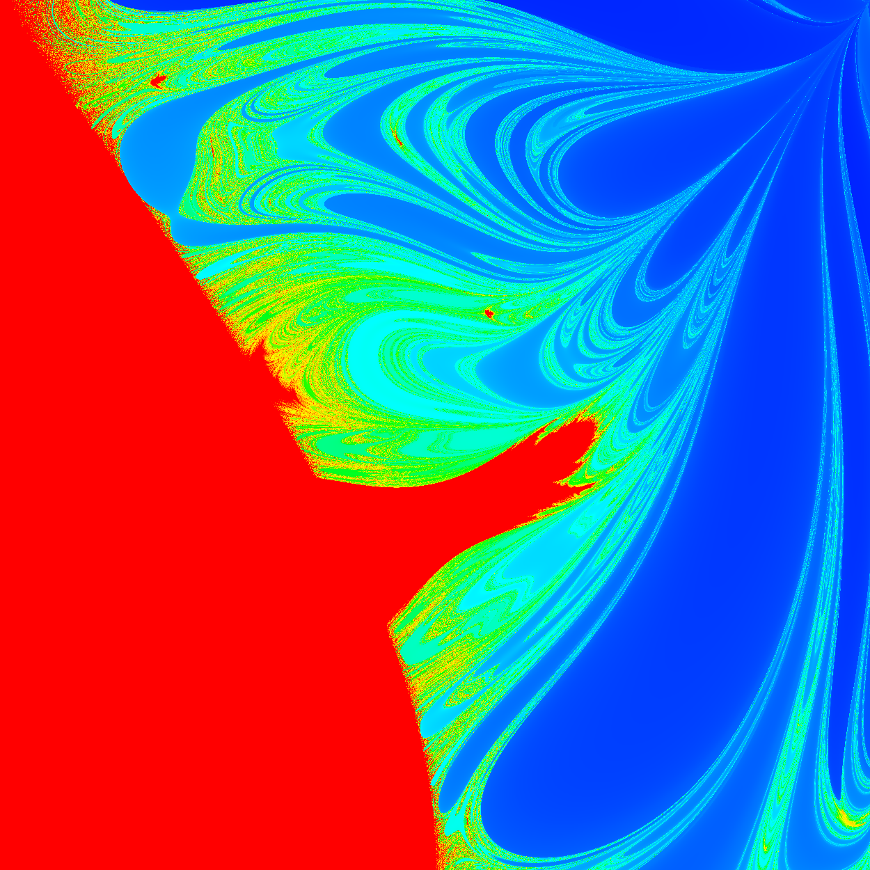
The warmer colors like reds and yellows indicate a longer time to flip and cooler colors like blues and greens indicate a shorter time. There are some interesting things in this image. First of all, the big red chunk in the bottom left quadrant. We can actually deduce this exact region mathematically, since in this area there is not enough energy for the pendulum to flip no matter how long the simulation runs. In fact, one little optimization I’ve done in the code is to not run the simulation if we are in this region - which is when 3cosθ1 + cosθ2 > 2.
//check if there is enough energy for a flip; if not, the skip to the next iteration
if (3*cos(a) + cos(c) > 2) {
    *(time_taken + j*n + i) = max_time + h;
    continue;
}
Furthermore, there seem to be “smooth” and “rough” areas. When zooming in on the rough areas, we typically see smaller and smaller stripes until it gets too grainy to distinguish. A certain initial position may flip very shortly, while a position infinitesimally similar may take much longer to flip. This is a fractal-like pattern. Meanwhile, the smooth areas imply that neighborhoods of initial conditions there yield non-chaotic pendulum motion, at least temporarily. A further analysis of what regions are where and what they indicate, as well as where the pendulum will definitely flip and where it won’t, is needed.
Lastly, I’ve included a second routine in the file error_graph.c. This method generates a similar graph but rather than timing the first flip of the pendulum, it runs the simulation for the full time allowed and calculates the final energy error. Since this system is chaotic, and we are using an approximate method, we know that after a certain amount of time our simulation is useless. We have no way of knowing how far our solution is from the unknown true position of the pendulum. However, we can calculate the energy precisely at every position. If the energy of our system changes drastically, this is an indicator that we’ve deviated far from the true solution. However, this is a very hacked and imprecise assessment since two very different positions/velocities may have similar total energies. Either way, knowing where the energy deviates may be interesting.