Neural Style Transfer

Introduction

Neural style transfer is the idea of reproducing any image in the style of a chosen piece of 2d artwork. The algorithm takes a content image, which is usually a photo, and a style image, which is usually a hand-created art piece. It then reproduces the content image in the style extracted from the style image using a neural network.

As an example, here is a picture of a mountain reproduced in the same style as The Scream by Edvard Munch.


The content image.


The style image.


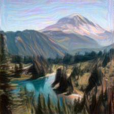
The output image.

The algorithm I implemented was described in the 2016 paper “A Neural Algorithm of Artistic Style”. by Gatys et. al. It uses the pre-trained VGG19 network. VGG19 is a 19-layer convolutional neural network which won the ImageNet Large-Scale Visual Recognition Challenge in 2014. In that sense, it is a successor of AlexNet, a very famous neural network which won in 2012.

Implementation details

Now, I’ll break down the most important parts of the code for this project. I won’t go through every line for the sake of brevity, but will go over the most important parts. First of all, to run this, we need the following imports:

import matplotlib.pyplot as plt
from PIL import Image
import torch
from torchvision import transforms, models
import numpy as np
from torch import optim

Next, we download the VGG19 model and put it on our device (which can be a cpu or gpu(CUDA)). We also freeze the model, which means that we aren’t actually back-propping on the weights and biases of the model, since it is already trained.

# Get the original VGG net model (only the feature extraction layers)
vgg19 = models.vgg19(pretrained=True).features
vgg19.to(dev)

# Freeze the network parameters since it is pretrained and we aren't transfer learning
for param in vgg19.parameters():
    param.requires_grad_(False)

After this I defined a load_image function, which simply scales and normalizes the input images and makes them into tensors. All images have to be 224x224 RGB for VGG19. It’s the first function I called after defining the path to each image (which must be in the same directory as the project root).

Here’s an important function:

def get_features(image, model, layers=None):
    """
    Run an image forward through a model and get the features for a set of layers.
    """

    # Label the relevant layers that can be used for style and content
    if layers is None:
        layers = {'0': 'conv1_1',
                  '5': 'conv2_1',
                  '10': 'conv3_1',
                  '19': 'conv4_1',
                  '21': 'conv4_2',
                  '28': 'conv5_1'}

    features = {}
    x = image
    # model._modules is a dictionary holding each module in the model
    for name, layer in model._modules.items():
        x = layer(x)
        if name in layers:
            features[layers[name]] = x

    return features

This function takes an image, forward-propagates it through the model (up until the linear classification layers, since those do not extract features), and returns a dictionary with features from the selected layers. These are the layers that are used in the paper. It may be worth experimenting with other layers, and this is a simple change requiring changing only the “layers” dictionary here and the “style_weights” dictionary later in the program.

# Experiment with values, and can add layers.
style_weights = {'conv1_1': 1.0,
                 'conv2_1': 0.8,
                 'conv3_1': 0.4,
                 'conv4_1': 0.2,
                 'conv5_1': 0.1}

The last central function in this script is the gram_matrix function.

def gram_matrix(tensor):
    # Ignore batch size since it is 1 in this case
    _, c, h, w = tensor.shape

    # Vectorize the feature, c is the channel count or "depth"
    tensor_v = tensor.view(c, h*w)

    # Compute the gram matrix
    gram = torch.mm(tensor_v, tensor_v.transpose(0, 1))

    return gram

This creates a gram matrix for a specific feature layer. This one is a little hard to visualize, but it essentially stores the similarity of each filter with each other filter in the layer. Here is the equation for each element of the gram matrix.

You will notice that the gram matrix contains the dot product of each row with each other row in the vectorized feature layer. The dot product is a great measure of similarity between vectors. The gram matrix is used specifically to calculate the style of an image. Simply using the feature layer isn’t enough since location, size, rotation, and other aspects aren’t important for style. On the other hand, for the content, these things are all retained. You can see this in action in our loop.

Our initial output starts as the content image itself. We could also start with a random image, but according to intuition and experimentation starting with the content image will get us there much faster since much of the work has already been done.

# The image we are generating
target_image = content_image.clone().requires_grad_(True).to(dev)

Training the Model

First, we get the target features using our get_features function, including the style and content layers.

target_features = get_features(target_image, vgg19)

Then, we get the content loss. There is a separate content loss and style loss, and we combine them since we want to match each one. We can arbitrarily choose the weights of the content vs. the style which determines which takes precedence. A content-heavy loss will mainly reproduce the content image with only minor style alterations. A style-heavy loss will greatly manipulate the content image until it is unrecognizable. A good balance is needed here.

The Content Loss.

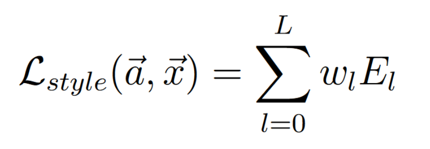
The Style Loss.
Here are the loss equations in action:

content_loss = torch.mean((content_features['conv4_2'] - target_features['conv4_2'])**2)

#initialize the style loss
style_loss = 0

# Weighted sum of the target style gram matrices
for layer in style_weights:
    _, c, h, w = target_features[layer].shape
    style_loss += (1 / (4 * h * h * w * w)) * style_weights[layer] * torch.mean((gram_matrix(style_features[layer]) - gram_matrix(target_features[layer]))**2)

As you can see, we only use one layer for content and use several for style. This is experimentally deduced but is suggested by the paper. The content layer seems somewhat arbitrary, but the style layers are sensitive. Layers further down the network grasp more abstract and complex shapes, while earlier layers detect simple shapes like lines or small brush-strokes. Experimenting with the style_weights dictionary (also a hyperparameter) will affect how the style is extracted.

Lastly, we add up the content and style losses and back-propogate.

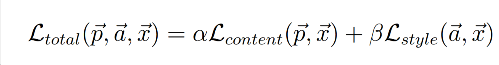
The Total Loss.

total_loss = content_weight * content_loss + style_weight * style_loss

optimizer.zero_grad()
total_loss.backward()
optimizer.step()

This loop runs for however many iterations you prefer. This, of course, depends on the learning rate. I used a learning rate of .003 for this. 500 iterations brings the majority of change, and 2000 should be enough for a final product.

Future Plans

Firstly, I am working on running this on a Google compute VM so I can use PyTorch + CUDA on their NVIDIA GPUs. This will be useful for generating many more examples efficiently. Currently the algorithm takes several minutes running on a laptop with i5 and no GPU.

After successfully completing that, I may choose to deploy this as a web app, if time permits.